Deep Residual Shrinkage Network: An Artificial Intelligence Method for Highly Noisy Data

The Deep Residual Shrinkage Network is an improved variant of the Deep Residual Network. Essentially, it is an integration of the Deep Residual Network, attention mechanisms, and soft thresholding functions.

To a certain extent, the working principle of the Deep Residual Shrinkage Network can be understood as follows: it utilizes attention mechanisms to identify unimportant features and employs soft thresholding functions to set them to zero; conversely, it identifies important features and retains them. This process enhances the deep neural network’s ability to extract useful features from signals containing noise.

1. Research Motivation

First, when classifying samples, the presence of noise—such as Gaussian noise, pink noise, and Laplacian noise—is inevitable. More broadly, samples often contain information irrelevant to the current classification task, which can also be interpreted as noise. This noise may negatively affect classification performance. (Soft thresholding is a key step in many signal denoising algorithms.)

For example, during a conversation by a roadside, the audio may be mixed with the sounds of car horns and wheels. When performing speech recognition on these signals, the results will inevitably be affected by these background sounds. From a deep learning perspective, the features corresponding to the horns and wheels should be eliminated within the deep neural network to prevent them from affecting the speech recognition results.

Secondly, even within the same dataset, the amount of noise often varies from sample to sample. (This shares similarities with attention mechanisms; taking an image dataset as an example, the location of the target object may differ across images, and attention mechanisms can focus on the specific location of the target object in each image.)

For instance, when training a cat-and-dog classifier, consider five images labeled as “dog.” The first image might contain a dog and a mouse, the second a dog and a goose, the third a dog and a chicken, the fourth a dog and a donkey, and the fifth a dog and a duck. During training, the classifier will inevitably be subject to interference from irrelevant objects such as mice, geese, chickens, donkeys, and ducks, resulting in a decrease in classification accuracy. If we can identify these irrelevant objects—the mice, geese, chickens, donkeys, and ducks—and eliminate their corresponding features, it is possible to improve the accuracy of the cat-and-dog classifier.

2. Soft Thresholding

Soft thresholding is a core step in many signal denoising algorithms. It eliminates features whose absolute values are lower than a certain threshold and shrinks features whose absolute values are higher than this threshold towards zero. It can be implemented using the following formula:

The derivative of the soft thresholding output with respect to the input is:

As shown above, the derivative of soft thresholding is either 1 or 0. This property is identical to that of the ReLU activation function. Therefore, soft thresholding can also reduce the risk of deep learning algorithms encountering gradient vanishing and gradient exploding.

In the soft thresholding function, the setting of the threshold must satisfy two conditions: first, the threshold must be a positive number; second, the threshold cannot exceed the maximum value of the input signal, otherwise the output will be entirely zero.

Additionally, it is preferable for the threshold to satisfy a third condition: each sample should have its own independent threshold based on its noise content.

This is because the noise content often varies among samples. For example, it is common within the same dataset for Sample A to contain less noise while Sample B contains more noise. In this case, when performing soft thresholding in a denoising algorithm, Sample A should utilize a smaller threshold, whereas Sample B should utilize a larger threshold. Although these features and thresholds lose their explicit physical definitions in deep neural networks, the basic underlying logic remains the same. In other words, each sample should have its own independent threshold determined by its specific noise content.

3. Attention Mechanism

Attention mechanisms are relatively easy to understand in the field of computer vision. The visual systems of animals can distinguish targets by rapidly scanning the entire area, subsequently focusing attention on the target object to extract more details while suppressing irrelevant information. For specifics, please refer to literature regarding attention mechanisms.

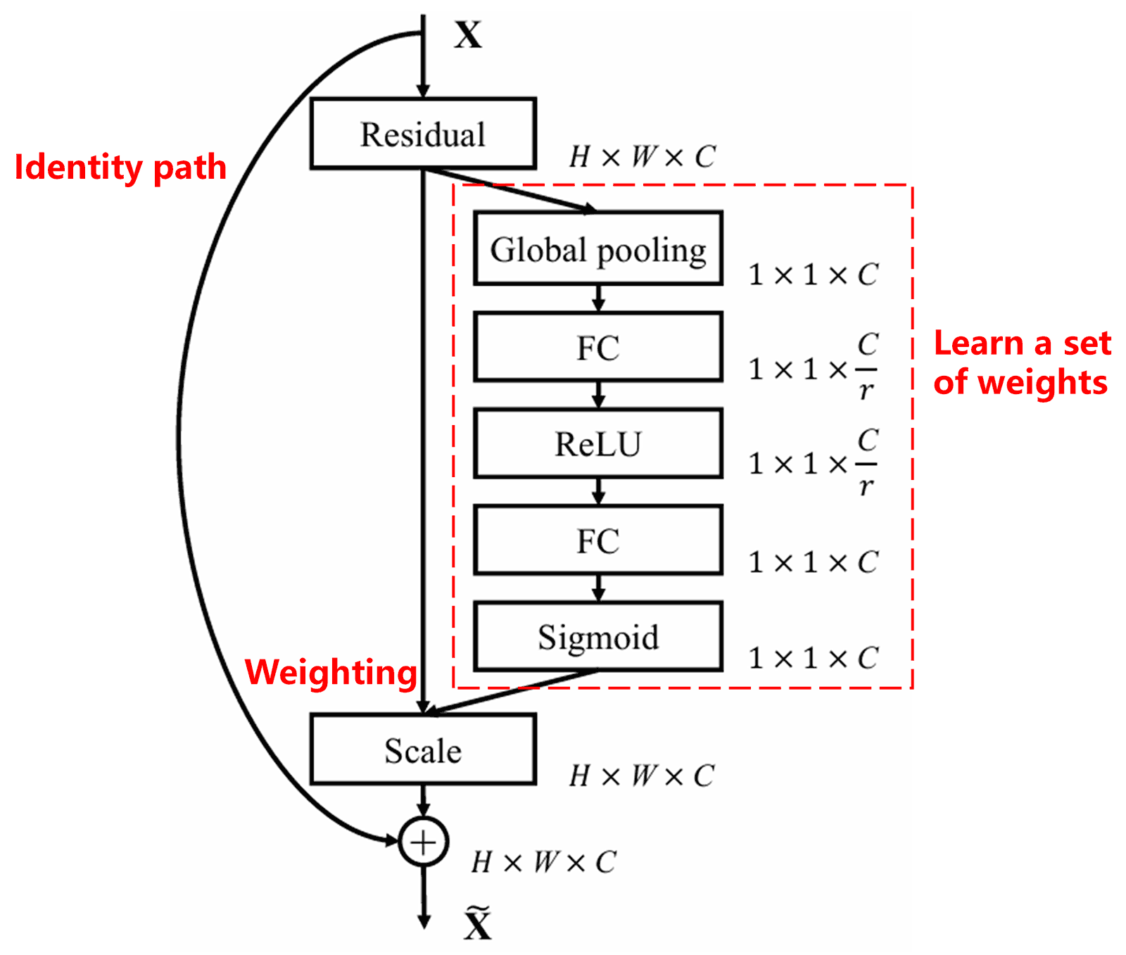
The Squeeze-and-Excitation Network (SENet) represents a relatively new deep learning method utilizing attention mechanisms. Across different samples, the contribution of different feature channels to the classification task often varies. SENet employs a small sub-network to obtain a set of weights and then multiplies these weights by the features of the respective channels to adjust the magnitude of the features in each channel. This process can be viewed as applying varying levels of attention to different feature channels.

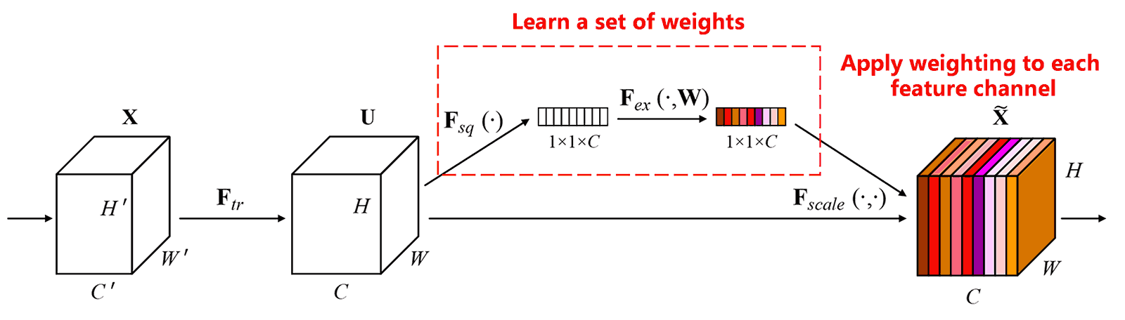
In this approach, every sample possesses its own independent set of weights. In other words, the weights for any two arbitrary samples are different. In SENet, the specific path for obtaining weights is “Global Pooling → Fully Connected Layer → ReLU Function → Fully Connected Layer → Sigmoid Function.”

4. Soft Thresholding with Deep Attention Mechanism

The Deep Residual Shrinkage Network draws inspiration from the aforementioned SENet sub-network structure to implement soft thresholding under a deep attention mechanism. Through the sub-network (indicated within the red box), a set of thresholds can be learned to apply soft thresholding to each feature channel.

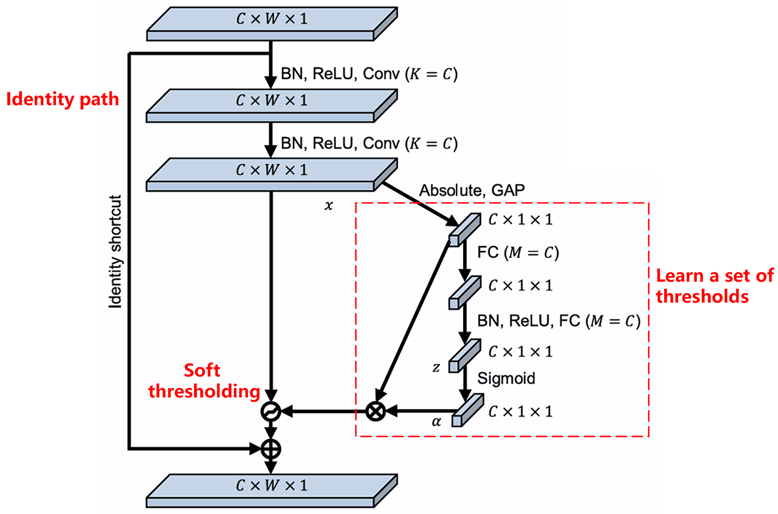
In this sub-network, the absolute values of all features in the input feature map are first calculated. Then, through global average pooling and averaging, a feature is obtained, denoted as A. In the other path, the feature map after global average pooling is input into a small fully connected network. This fully connected network uses the Sigmoid function as its final layer to normalize the output between 0 and 1, yielding a coefficient denoted as α. The final threshold can be expressed as α×A. Therefore, the threshold is the product of a number between 0 and 1 and the average of the absolute values of the feature map. This method ensures that the threshold is not only positive but also not excessively large.

Furthermore, different samples result in different thresholds. Consequently, to a certain extent, this can be interpreted as a specialized attention mechanism: it identifies features irrelevant to the current task, transforms them into values close to zero via two convolutional layers, and sets them to zero using soft thresholding; alternatively, it identifies features relevant to the current task, transforms them into values far from zero via two convolutional layers, and preserves them.

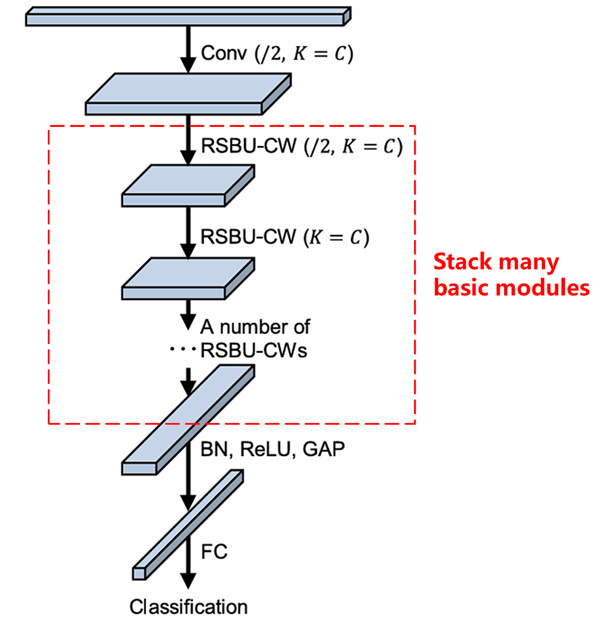
Finally, by stacking a certain number of basic modules along with convolutional layers, batch normalization, activation functions, global average pooling, and fully connected output layers, the complete Deep Residual Shrinkage Network is constructed.

5. Generalization Capability

The Deep Residual Shrinkage Network is, in fact, a general feature learning method. This is because, in many feature learning tasks, samples more or less contain some noise as well as irrelevant information. This noise and irrelevant information may affect the performance of feature learning. For example:

In image classification, if an image simultaneously contains many other objects, these objects can be understood as “noise.” The Deep Residual Shrinkage Network may be able to utilize the attention mechanism to notice this “noise” and then employ soft thresholding to set the features corresponding to this “noise” to zero, thereby potentially improving image classification accuracy.

In speech recognition, specifically in relatively noisy environments such as conversational settings by a roadside or inside a factory workshop, the Deep Residual Shrinkage Network may improve speech recognition accuracy, or at the very least, offer a methodology capable of improving speech recognition accuracy.

Reference

Minghang Zhao, Shisheng Zhong, Xuyun Fu, Baoping Tang, Michael Pecht, Deep residual shrinkage networks for fault diagnosis, IEEE Transactions on Industrial Informatics, 2020, 16(7): 4681-4690.

https://ieeexplore.ieee.org/document/8850096

BibTeX

@article{Zhao2020,
  author    = {Minghang Zhao and Shisheng Zhong and Xuyun Fu and Baoping Tang and Michael Pecht},
  title     = {Deep Residual Shrinkage Networks for Fault Diagnosis},
  journal   = {IEEE Transactions on Industrial Informatics},
  year      = {2020},
  volume    = {16},
  number    = {7},
  pages     = {4681-4690},
  doi       = {10.1109/TII.2019.2943898}
}

Academic Impact

This paper has received over 1,400 citations on Google Scholar.

According to conservative estimates, Deep Residual Shrinkage Networks (DRSN) have been utilized in more than 1,000 publications. These works have either directly applied or improved upon the network across a wide range of fields, including mechanical engineering, electric power, computer vision, healthcare, speech processing, text analysis, radar, and remote sensing.